Clock Discipline Before Correlation: A Timestamp Audit for Test and Simulation

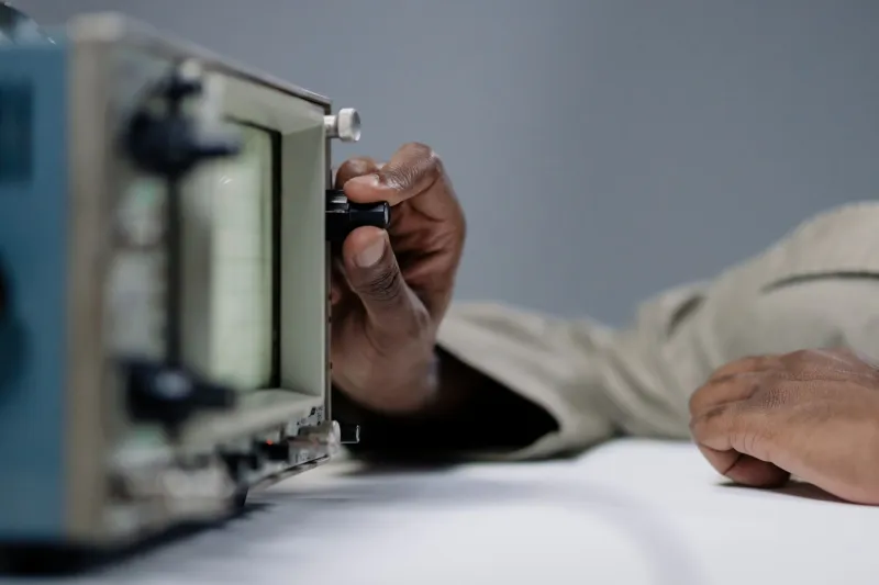
At the correlation review, the first question is usually about boundary conditions, damping, or mesh density. The clock rarely comes up. Yet a single timestamp offset of 40 milliseconds can rotate phase enough to make a defensible model look wrong, and a one-hour daylight-saving error can make a good test look like a different test altogether. Time alignment is not metadata hygiene. It is an engineering tolerance, and it deserves a budget, a verification method, and a place in the handoff file.

Time Is a Tolerance, Not a Footnote

A tolerance is a permissible deviation with a stated verification method. Timestamps have bias, drift, resolution, and ambiguity. Each of those quantities can be measured. Each can be bounded. The trouble starts when teams treat the time column as ground truth because it came from a data acquisition system or a solver output file.

Consider phase. A 10-millisecond timing offset produces 18 degrees of phase error at 5 Hz and 180 degrees at 50 Hz. If the correlation target is phase agreement within 5 degrees at 20 Hz, the allowable timestamp offset is roughly 0.7 milliseconds. That number belongs in the test plan next to the accelerometer range and the sampling bandwidth. It does not belong in a post-mortem after the model has been blamed for a clock problem.

Four Ways Correlation Loses Time

Clock skew between subsystems. The DAQ, the real-time controller, the host PC, and the network switch may each keep their own notion of time. Host-level NTP synchronization can wander by tens of milliseconds under load. That is adequate for file timestamps and inadequate for modal correlation. If the test article and the simulation share an event, they need a shared time base, not four reasonable approximations.

Local time and daylight-saving transitions. The United States still observes daylight-saving time in most states, and the November fallback creates a duplicated local hour. A file written in local time without an explicit UTC offset is ambiguous for one hour each year. A one-hour error does not look like a clock problem in a plot; it looks like a completely different operating condition. Store UTC with an explicit offset, and keep the time-zone rules with the data.

Sample-rate error. A DAQ specified at 1,000 Hz may run at 999.98 Hz because the oscillator is not perfect. Twenty parts per million sounds harmless until a ten-minute capture accumulates about 12 milliseconds of drift relative to a perfect clock. At 50 ppm, the same capture drifts about 30 milliseconds. Nominal sample rate is a label. Actual sample rate is a measurement, and it should be logged with a frequency counter or a known reference signal.

Solver time metadata. Simulation output may report physical time, iteration count, CPU time, or an output interval that was interpolated from internal steps. Restart files can carry a different zero. A correlation script that assumes the first column is physical seconds will silently mix time bases. The solver deck should state what the time column means, how output was sampled, and whether interpolation was applied.

A Timestamp Audit Checklist

1. Inventory every clock in the measurement chain: sensors, DAQ, real-time controller, host workstation, network switch, cameras, and the solver machine.
2. Record the time source for each device: GPS, PTP, NTP, free-run oscillator, or manual entry.
3. Measure offset and drift at the start and end of each run using a common hardware trigger, pulse-per-second signal, or IRIG-B reference where available.
4. Store raw timestamps in UTC using ISO 8601 with an explicit offset. Ban local-time-only timestamps in raw data files.
5. Verify actual sample rates against nominal values and log the measured rate, not the requested rate.
6. Confirm the meaning of the solver time column: physical time, step index, output interval, or interpolated sample.
7. Prefer hardware triggers over software events for the correlation reference.
8. Document the interpolation method used to compare test and simulation samples.
9. Calculate a time-error budget for the correlation and compare it with the phase tolerance.
10. Include a clock log in the test report and the correlation package.

A Defensible Time-Sync Protocol

A practical protocol has tiers. At the top, hardware synchronization such as IEEE 1588 precision time protocol or a shared trigger and clock distribution provides sub-millisecond alignment. In the middle, NTP with continuous offset monitoring can support lower-frequency correlation if the measured error is inside the budget. At the bottom, free-run clocks are acceptable only when drift is measured and corrected in post-processing, and the correction method is documented.

For US teams, internet time services are convenient but not a defensible sole reference for a design-review correlation. A local GPS-disciplined oscillator or a facility time server with logged offset history is easier to audit. The acceptance criterion should be written before the test: for example, timestamp offset below 1 millisecond and drift below 10 parts per million across the capture. Then the correlation report can state that the time base met its tolerance rather than assuming it did.

The Handoff File

The correlation handoff should include a time manifest alongside the test data and the simulation deck. The manifest should state the time source, synchronization status, measured offset, drift rate, actual sample rate, trigger timestamp, time-zone rules, and the meaning of every time column in the solver output. A machine-readable sidecar file is better than a note in an email because the correlation script can read it instead of guessing.

When the model and the test disagree, the review will look for a culprit. Bad physics is a plausible defendant. Bad clocks are a quieter one. Before the model stands trial, cross-examine the time base. If the timestamps are not under control, the correlation is not measuring what the team thinks it is measuring.